
Detecting Pulsars
I found this dataset for pulsars on kaggle. The data is a sample from data collected during the High Time Resolution Universe Survey. Pulsars can be hard to detect because of radio frequency interference (RFI) and noise. I wanted to see how well I could detect pulsars in this imbalanced dataset using logistic regression. I could have used more sophisticated methods such as random forests and support vector machines, but I wanted to see how well a simplier model worked. The dataset is descibed below.
- Mean of the integrated profile.
- Standard deviation of the integrated profile.
- Excess kurtosis of the integrated profile.
- Skewness of the integrated profile.
- Mean of the DM-SNR curve.
- Standard deviation of the DM-SNR curve.
- Excess kurtosis of the DM-SNR curve.
- Skewness of the DM-SNR curve.
- Class
%matplotlib inline
import numpy as np
import pandas as pd
import matplotlib.pyplot as plt
from sklearn.model_selection import train_test_split
import seaborn as sns
from sklearn.preprocessing import StandardScaler, PowerTransformer, PolynomialFeatures
import statsmodels.api as sm
from sklearn.metrics import confusion_matrix, roc_curve, roc_auc_score
from sklearn.linear_model import LogisticRegression, LogisticRegressionCV
from sklearn.ensemble import RandomForestClassifier
from sklearn.pipeline import Pipeline
from sklearn.compose import ColumnTransformer
from sklearn.feature_selection import RFECV
from sklearn.svm import SVC
from sklearn.decomposition import PCA
from typing import Tuple
random_state = 42
FIGSIZE = (9, 6)
FONTSIZE = 14
def read_data(filename: str) -> Tuple:
    all_data = pd.read_csv(filename, delimiter=',',header=0,
                       names=['Mean', 'Std', 'Kurtosis', 'Skewness',
                              'Mean DM-SNR', 'Std DM-SNR', 'Kurtosis DM-SNR',
                              'Skewness DM-SNR', 'target'])
    y = all_data['target']
    X = all_data.drop('target', axis=1)
    return X, y
def class_imbalance_calculator(y):
    return np.sum(y) / len(y)
X, y = read_data('pulsar_stars.csv')
imbalance = class_imbalance_calculator(y)
print(f"Overall class imbalance: {imbalance*100:3.2f}%")
Overall class imbalance: 9.16%
X_train, X_test, y_train, y_test = train_test_split(X, y, random_state=random_state)
X_train, X_valid, y_train, y_valid = train_test_split(X_train, y_train, random_state=random_state)
print(f"Train class imbalance: {class_imbalance_calculator(y_train)*100:3.2f}%")
print(f"Validation class imbalance: {class_imbalance_calculator(y_valid)*100:3.2f}%")
print(f"Test class imbalance: {class_imbalance_calculator(y_test)*100:3.2f}%")
Train class imbalance: 9.17%
Validation class imbalance: 9.27%
Test class imbalance: 9.05%
def create_logistic_regression_pipeline(log_features: list, standard_features: list) -> Pipeline:
    """Create a logistic regression classifier pipeline

    Creates a logistic regression classifier pipeline. Any features that are not listed in log_features and standard_features
    at the time of fitting will be dropped.

    :param log_features: column names that the PowerTransformer will be applied to
    :param standard_features: column names that the StandardScaler will be applied to
    :return: a scikit-learn pipeline that transforms the data and has a LogisticRegressionCV
    :rtype Pipeline
    """
    preprocessor = ColumnTransformer(
        transformers=[
            ('log_normal', PowerTransformer(method='yeo-johnson', standardize=True), log_features),
            ('normal', StandardScaler(), standard_features)], remainder='drop')
    clf = Pipeline(steps=[
                  ('preprocessing', preprocessor),
                  ('classifier', LogisticRegressionCV(
                      random_state=random_state, Cs=10, cv=5, class_weight='balanced',
                      scoring='recall',
                  )),
                   ])
    return clf
What results can we get using all columns with just standard scaling with some regularization chosen by cross validation?
clf_no_log_features = create_logistic_regression_pipeline([], X_train.columns)
clf_no_log_features.fit(X_train, y_train)
y_valid_predict = clf_no_log_features.predict(X_valid)
conf_mat = confusion_matrix(y_valid, y_valid_predict)
print(conf_mat)
tp = conf_mat[1, 1]
tn = conf_mat[0, 0]
fn = conf_mat[1, 0]
fp = conf_mat[0, 1]
print(f"Recall: {tp / (tp + fn)}")
print(f"Precision: {tp / (tp + fp)}")
[[2971   74]
 [  28  283]]
Recall: 0.909967845659164
Precision: 0.7927170868347339
Let’s examine what our feature matrix looks like and see if we should use a different scaling
# full_df = pd.concat([X_train, y_train.reset_index(drop=True)], axis=1)
# sns.pairplot(full_df, hue='target', vars=X_train.columns)
_=pd.plotting.scatter_matrix(X_train, figsize=(10,10))
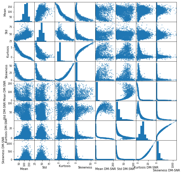
It looks like the columns that we don’t need to do anything with are mean Std, and Kurtosis DM-SNR. The rest I think require a log transform.
log_features = ['Kurtosis', 'Skewness', 'Mean DM-SNR', 'Std DM-SNR', 'Skewness DM-SNR']
standard_features = ['Mean', 'Std', 'Kurtosis DM-SNR']
clf_with_log_features = create_logistic_regression_pipeline(log_features, standard_features)

preprocessor = clf_with_log_features.named_steps['preprocessing']
preprocessor.fit(X_train)
X_train_transformed = preprocessor.transform(X_train)
X_train_transformed_df = pd.DataFrame(X_train_transformed, columns=log_features+standard_features)
_=pd.plotting.scatter_matrix(X_train_transformed_df, figsize=(10,10))
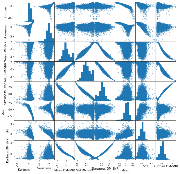
Now the columns are looking closer to Gaussian, let’s try fitting with all columns and regularization
clf_with_log_features.fit(X_train, y_train)
y_valid_predict = clf_with_log_features.predict(X_valid)
conf_mat = confusion_matrix(y_valid, y_valid_predict)
print(conf_mat)
tp = conf_mat[1, 1]
tn = conf_mat[0, 0]
fn = conf_mat[1, 0]
fp = conf_mat[0, 1]
print(f"Recall: {tp / (tp + fn)}")
print(f"Precision: {tp / (tp + fp)}")
[[2921  124]
 [  26  285]]
Recall: 0.9163987138263665
Precision: 0.6968215158924206
Adding log features increased our recall but decreased our precision some.
It is worth noting that there are definitely some strong correlations in the data. What if we removed some of the strongest correlations. Let’s try removing Std DM-SNR, Skewness DM-SNR, and Kurtosis DM-SNR
log_features = ['Kurtosis', 'Skewness', 'Mean DM-SNR']
standard_features = ['Mean', 'Std']

clf_log_reg = create_logistic_regression_pipeline(log_features, standard_features)

preprocessor = clf_log_reg.named_steps['preprocessing']
preprocessor.fit(X_train)
X_train_transformed = preprocessor.transform(X_train)
X_train_transformed_df = pd.DataFrame(X_train_transformed, columns=log_features+standard_features)
_=pd.plotting.scatter_matrix(X_train_transformed_df, figsize=(10,10))
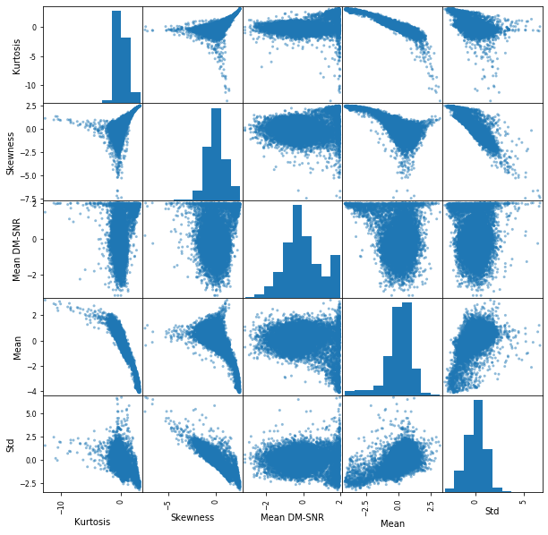
There are still some correlations, but not as drastic as before. Let’s see how the new model performs.
clf_log_reg.fit(X_train, y_train)
y_valid_predict = clf_log_reg.predict(X_valid)
conf_mat = confusion_matrix(y_valid, y_valid_predict)
print(conf_mat)
tp = conf_mat[1, 1]
tn = conf_mat[0, 0]
fn = conf_mat[1, 0]
fp = conf_mat[0, 1]
print(f"Recall: {tp / (tp + fn)}")
print(f"Precision: {tp / (tp + fp)}")
[[2953   92]
 [  26  285]]
Recall: 0.9163987138263665
Precision: 0.7559681697612732
Our recall stayed the same, but we have an increase in the precision.
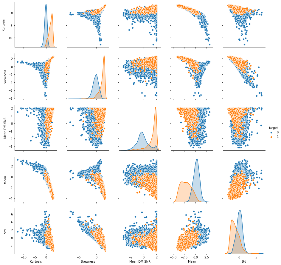
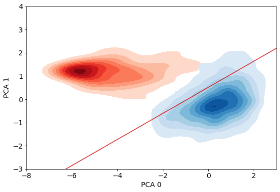
Let’s try to visualize how well our logistic regression is doing visually by using principal component analysis
columns = ['Kurtosis', 'Skewness', 'Mean DM-SNR', 'Mean', 'Std']
x_transformer = clf_log_reg.named_steps['preprocessing']
x_train_transformed = x_transformer.transform(X_train)
x_train_transformed_df = pd.DataFrame(x_train_transformed, columns=columns)
full_df = pd.concat([x_train_transformed_df, y_train.reset_index(drop=True)], axis=1)
_ = sns.pairplot(full_df, hue='target', vars=columns)
pca_dim = 2
pca = PCA(n_components=pca_dim, random_state=random_state)
pca.fit(x_train_transformed)
print(f"{sum(pca.explained_variance_ratio_)*100}% of the variance in the data is explained by the first two pricipal components")
82.46593032331847% of the variance in the data is explained by the first two pricipal components
x_valid_transformed = x_transformer.transform(X_valid)
# x_pca = pca.transform(x_train_transformed)
x_pca = pca.transform(x_valid_transformed)

x_pca_df = pd.DataFrame(x_pca, columns=range(pca_dim))

# full_df = pd.concat([x_pca_df, y_train.reset_index(drop=True)], axis=1)
full_df = pd.concat([x_pca_df, y_valid.reset_index(drop=True)], axis=1)
log_reg_classifier = clf_log_reg.named_steps['classifier']
log_reg_coeff = log_reg_classifier.coef_[0]
log_reg_intercept = log_reg_classifier.intercept_[0]

npts = 100
x = np.zeros((npts, 5))
for i in range(4):
    x[:, i] = np.linspace(x_pca.min(), x_pca.max(), npts)

x[:, 4] = (0.5 - log_reg_intercept - np.sum((log_reg_coeff*x)[:, 0:4], axis=1) )/ log_reg_coeff[-1]

xx = pca.transform(x)

fig, ax  = plt.subplots(figsize=FIGSIZE)
sns.kdeplot(data=full_df[full_df['target']==1].loc[:, 0], data2=full_df[full_df['target']==1].loc[:, 1],
            cmap='Reds', shade=True, shade_lowest=False)
sns.kdeplot(data=full_df[full_df['target']==0].loc[:, 0], data2=full_df[full_df['target']==0].loc[:, 1],
            cmap='Blues', shade=True, shade_lowest=False)

i = np.abs(xx[:, 0]+8).argmin()
j = np.abs(xx[:, 0]-3).argmin()
if i>j:
    i, j = j, i
ax.plot(xx[i:j, 0], xx[i:j, 1], '-', color='C3')

ax.set_xlim(-8, 3)
ax.set_ylim(-3, 4)
ax.tick_params(labelsize=FONTSIZE)
ax.set_xlabel("PCA 0", fontsize=FONTSIZE)
ax.set_ylabel("PCA 1", fontsize=FONTSIZE)

plt.show()
How well does our model perform on the test set?
Overall, I think our model performs reasonably well on predicting pulsars. The goal is to try to pick out candidates that can be further examined by trained eyes.
We could possibly lower the recall but at the cost of the precision. We could possibly rerun the training with the goal of maximizing the f1 score as opposed to recall. It might make a slightly better trade off between recall and precision.
y_test_predict = clf_log_reg.predict(X_test)
conf_mat = confusion_matrix(y_test, y_test_predict)
print(conf_mat)
tp = conf_mat[1, 1]
tn = conf_mat[0, 0]
fn = conf_mat[1, 0]
fp = conf_mat[0, 1]
print(f"Recall: {tp / (tp + fn)}")
print(f"Precision: {tp / (tp + fp)}")
[[3948  122]
 [  30  375]]
Recall: 0.9259259259259259
Precision: 0.7545271629778671